Introduction

The Rose Range Lite (RRL) coloring formula is one of many I've written that colors the image according to how the pixel relates to a geometric figure. Here, I hope to explain how to use the formula effectively. As an example, we'll see how to create this basket.

Rose Curves

where N is the frequency of the cosine or sine function, typically an integer (e.g., 1, 2, 3, etc.). The difference between using the sin() or cos() functions is just a rotation. Strictly speaking, the r variable above is a true coordinate, not just a distance. This means that r can be negative. In RRL, r is implemented through the cabs() function, which will never give a negative result. Here, we see the differences between true rose curves and my versions (click on the image to download the upr):

On the left are true rose curves. The blue curve is r = cos(2q) and the red is r = sin(2q). Both are the same size and shape, the only difference is a rotation of 45 degrees. Notice that both curves have 4 lobes, or "petals." If N is an even integer (2, 4, 6, etc.), then the rose curve for cos(Nq) or sin(Nq) will have 2N petals. If N is odd, then its rose curve will have just N petals. The curves from RRL are shown on the right, for the same 2 equations. They only have 2 petals each, but the petals are the same size and shape and in the same location as the "real" curves. This is due to using the cabs() function and my formula not handling negative r values. For odd values of N, the formula will give the same number of petals as the real equation. (The image on the left was generated with a prototype formula that breaks each curve up into hundreds or thousands of points, then checks each pixel against each of the points on the curve. While more accurate, it is much, much slower than RRL, so I did not publish it.)

The other major difference between the left and right panels is that the RRL curves get vanishingly thin at the center, then nice and wide at the outer edges. This is because RRL is implemented as a range formula. When r is determined from the equation, then a range is specified above and below r. For example, if r = 1, then the range might be from 0.9 to 1.1. If the point falls in this range, then it is colored appropriately. The width of the range scales with r, for example it may be 10% of r. So, as r gets very small (in the center of the image), then the width of the range gets very small, and the curves get very thin.

For greater flexibility, I used both the sin() and cos() functions to determine r:

where A_c is the amplitude of the cosine portion of the curve and N_c is its frequency. A_s and N_s are the amplitude and frequency of the sine portions. Before we get into the details of making these curves, here are some examples (click on the image for the upr):
 

Ac = 1 Nc = 0 As = -0.5 Ns = 4

Ac = 1 Nc = 2 As = -1 Ns = 5

Ac = 0.5 Nc = 0 As = 1 Ns = 4.5

When N is not an integer, as in the last case, then the curve does not close. Normally, that's to be avoided, but we're going to use that feature to make the basket.

Tutorial

• Create a new fractal, using the Pixel formula from the mt folder.
• In the Location tab, set the Center to 0/0 and the Magnification to 1 (or just click the Reset Location icon in the lower right corner of the top Properties box).
• In the Formula tab, set:
• Drawing Method: Multi-pass Linear
• Periodicity Checking: Off
• Maximum Iterations: 1
• Adjust Automatically checkbox: doesn't matter, since we're only using 1 iteration.
• Inside: check the Enabled box

• Since all the pixels will be inside (that's why you checked the Enabled box in Step 1), there's nothing to do with the Outside tab.
• In the Inside tab, click on the Select icon (3 dots) and choose Rose Range Lite from the lkm folder. You should see a 3-petal rose curve.
• Set the Inside parameters:
• Color Density: 1
• Transfer Function: Linear
• Gradient Offset: 0
• Repeat Gradient checkbox: doesn't matter, checked or cleared
• Click the Reset Parameters icon in the lower right corner to reset all the formula-specific parameters.
• Set the "color by" formula parameter to "last magnitude."
• Click on the Solid Color icon (the black mini Mandelbrot shape on the right side of the top Properties box). Set the solid color to white (set the Luminance to 255).
• Set the gradient.
• Open the Gradient Editor and delete all the control points. Continue to click the Delete icon until there's only one left, a black control point at Index 0.
• Close the Gradient Editor.

• On the Layers tab of the lower Properties box, set the Width and Height parameter to the same values (say, 480 pixels). You may need to clear the Maintain aspect ratio box to do this.
• You should now have an image that looks like the one on the right. It's not much yet, but that's ok.  Click on the image to see the upr.

• In the Layers tab of the lower Properties box, change the Name of this layer to "New Layer 1." This will help keep things straight when we add 18 more layers.
• In the Location tab of the upper Properties box, change the Magnification to 1.2. Keep the Center at 0/0. Change the Rotation angle to 281.
• In the Inside tab, set the formula-specific parameters:
• range scale: 1
• range width: 0.02. This will make the line much thinner, so it's important to use Multi-pass Linear or One-pass Linear as the Drawing Method.
• color by: last magnitude
• cos amplitude: 1
• cos frequency: 0
• sin amplitude: 0.5
• sin frequency: 7.5. This will cause the line to open up and not close on itself.
• curve center: 0/0
• rotation angle: 0
• Compare your results with the figure on the left. If they match, proceed. If not, try to find and fix any errors, or use the upr (click on image).

• We need to close that curve and join up with those free ends. Click on the Add icon at the bottom of the Layers tab in the bottom Properties box. This should add a new layer, "New Layer 2." Since all the parameters for this layer are the same as for the previous layer, the overall image shouldn't change.
• Change the Merge mode to Darken and the Opacity to 100%. These won't change the appearance of the image, either. However, when we change the rose curve parameters, then we'll see a difference. Since the image is being rendered in pure black and pure white, we'll use the Darken Merge mode at 100% to make sure that all the lines show through evenly.
• In the Inside tab of New Layer 2, change the sin frequency to see if you can find something that will match up the loose ends from New Layer 1. Here's a hint: the sin frequency needs to be some integer plus 0.5. Here's what happens with (from left to right) settings of 5.5, 6.5, 8.5, and 9.5:

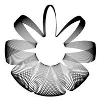
Now that we've seen how the basic process works, we're going to build the basket with 19 layers. We won't be particularly interested in the intermediate steps, and a 19 layer image can tax a system, so we'll build it small then survey our work later.

• In the Image tab of the bottom Properties box, check the Maintain aspect ratio box.
• Set the Width to something small, like 20. You won't be able to see what's happening with the image, but that's ok. We'll make it big when we're done.
• In the Inside tab of the top Properties box of New Layer 1 (the bottom layer), change the sin frequency to 7.1
• Change the sin frequency for New Layer 2 to 7.2.
• Make sure that New Layer 2 is highlighted in the Layers tab of the bottom Properties box. Click on the Add icon 17 times to add 17duplicate layers.
• Work up the stack from New Layer 2 to New Layer 19. Each layer should have its Merge mode set to Darken and Opacity set to 100%. The sin frequencies should increase by 0.1 each layer from 7.2 on New Layer 2 to 8.9 on New Layer 19. There should now be one layer (New Layer 10) with an integer sin frequency (8). The lower layers (1 - 9) have frequencies of 7.something. The upper layers (11 - 19) balance them out with frequencies of 8.something.
• When you've gotten everything set correctly, go back to the Image tab of the bottom Properties back and reset the width to 480 or something respectable. Depending on your system, it may take Ultra Fractal a while to organize itself, but the layers render pretty quickly. If you've made a mistake, it will probably show up as a gap between the otherwise regularly-spaced lines. The lines may appear broken if you use a small resolution. For best results, render it to disk with anti-aliasing.
• If all else fails, click on the basket below to see the upr.
• Enjoy your basket, and be sure to share your Rose Range Lite creations with the rest of the Ultra Fractal world!